Neural Networks: Introduction

To really understand neural networks,we first need to see what the how the most fundamental biological unit of our brain: Neuron works.

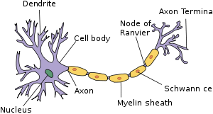
Each neuron is connected in one after the other with axon termina connected to the dendrite of the next neuron having a synaptic gap in between.These connections act as a transmission line.Human brain is estimated to have atleast 100 billion neurons.How can we model that sort of thing?

Scientists have tried modelling the neural network of a tapeworm which has just 302 neurons: Tapeworm Neural Model.

Human brain is indeed the most complex thing in the universe.You might thing A.I still has a long way to go before we could model a real human brain,which is somewhat true,but according to moore’s law,growth in any field is exponential after the initial growth spurt,as we have seen that computer speed nearly doubles after every two years.

DEMYSTIFYING NEURAL NETWORK:

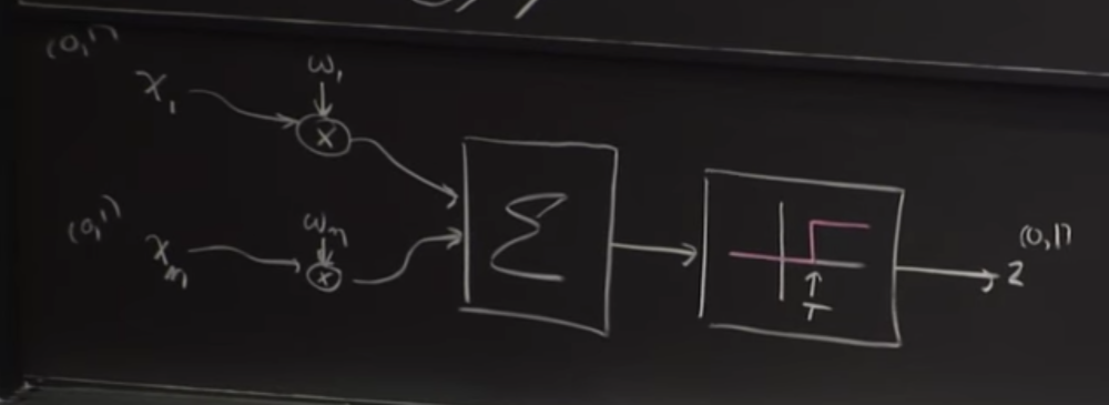
1. We have an input value X1,which is either a 0 or 1,which gets multiplied by some weight w1.
2. We have another input value X2,which is also either 0 or 1, which gets multiplied by weight w2.
3. These gets added in the form of cumulative effect summer,and the output from that is passes into a threshold box, which decides whether our final output is a 0 or 1.
4. If the threshold value is above some value output z is 1, otherwise output is 0.

In every neural network, the output z is a function of three factors,

z=ƒ(x,w,T): A neural net is a function approximator when you really think about it.

Here, z is what we get as output.Lets d be what we desire output to be.

d=ω(x).

So our desired output is is actually a function of our input x.We need to optimize the weights and threshold in such a way that our z is as closer to d as possible.

Let us define P as our performance parameter.

Here, P=-||d-z||²

The reason behind doing this is because ,we need a smooth graph(due to squaring) where reaching ‘0’ would be the zenith of our output,

Instead of this,

Consider this contour graph,

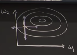
We have some weights w1 and w2 and we are trying to move in the direction of obtaining the best possible w1 and w2.

Instead of just trying out all possible values of w1 and w2,what we do is take partial derivate of our performance parameter P,with respect to w1 or w2. This would give the improvement that we are making with slight change of w1 or w2.

So the change would be,

Δw= r (δP/δ_w1 i+δP/δ_w2j).

‘r’ is going to determine how bigger our step would be.

This value Δw is going to our gradient ascent.

But the major problem faced here was gradient ascent of descent requires a continuous function but what we have here is nonlinear.

The entire progress in the field of neural networks was struck at this point for 25 years.

Until a solution was given by Paul Werbos in 1974 at Harvard.

Solution:

We would really like for thresholds to disappear because its just some extra baggage to deal with. We would rather have a function that looks like this: z=ƒ(x,w).

But we have to account for threshold somehow.

The Trick that was given by professor Werbos was to input another neuron ,say W0. Characteristics of this neuron w0 would be:

• W0 always has input value -1.
• Wo always has weight equal to threshold value T.

so ,W0 always produces -T for the summation chamber.What this does is that ,the system will produce the output z, if the summation of all inputs and wo is above 0.

This is how we get rid of threshold.

Another improvement that can be made is use of SIGMOD function:

Our threshold function was initially in the form of step function, we replace that with sigmoid function,which is a ‘s’ shaped curve. The sigmoid function is given as:

ƒ=1/(1+e^-α)

where α is the input.

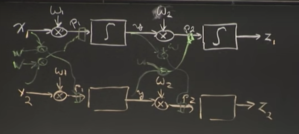
BUILDING A NEURAL NETWORK:

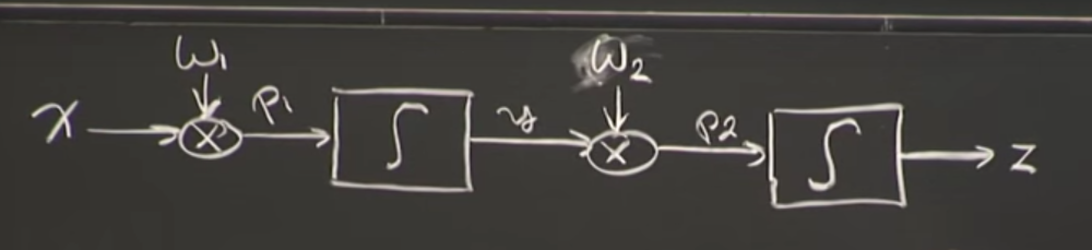
Let’s build a neural network consisting of two neurons,

Keeping performance parameter P as, P=-||d-z||² /2

We now need to calculate partial derivatives for change in values of w1 and w2,

Two parameters we have to calculate are, δP/δ_w1 and δP/δ_w2.

We need chain rule of derivatives for this, which essentially is,

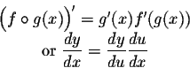
Complete chain rule article :here.

δP/δ_w2 = δP/δ_z*δz/δ_p2*δP2/δ_w2.(Chain rule applied!)   EQN[1]

δP/δ_w1 = δP/δ_z*δz/δ_p2*δP2/δ_y*δP2/δ_p1*δP1/δ_w1.(Chain rule applied!)    EQN[2]

All we need to do is find the partial derivatives,and we have our optimized required weights.

δP/δ_z : It is the derivative of performance parameter P with respect to z. Which is clearly equal to (d-z).

δP2/δ_w2:We can see from the image above that P2 is just y*w2,so its derivative with respect to w2 would be just y.

δz/δP2:We can observe that P2 is passing through the sigmoid function before giving output z.So we need to find derivative of the sigmoid function with respect to any input x.

Sigmoid function:ƒ=1/(1+e^-α).

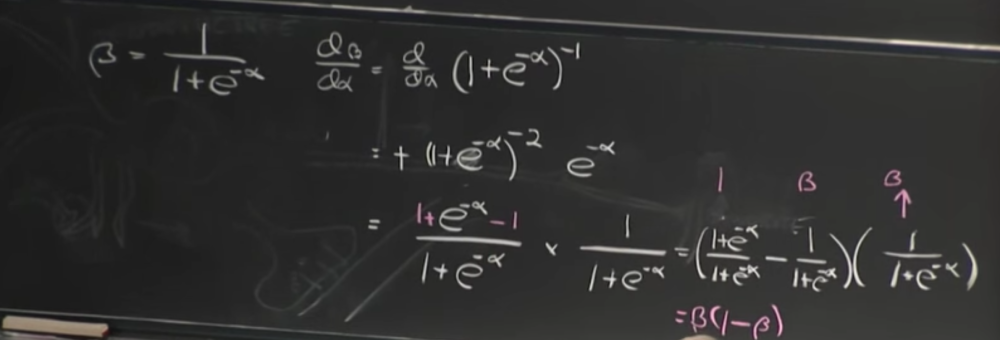
The derivative of output with respect to the input results in the value which is in terms of the output.In our case, output is z.

Therefore,δz/δP2=z(1-z).

For further understanding,

Consider a neural network with four neurons.

As you can see, there are connected pathways among neurons and you might think that number of pathways to obtain outputs are increased exponentially,which is true but the computations required has not grown exponentially, this is because,

When we see EQN[2], we observe that part of what has to be calculated is already done in EQN[1].

δP/δ_w2 = δP/δ_z*δz/δ_p2*δP2/δ_w2.

δP/δ_w1 = δP/δ_z*δz/δ_p2*δP2/δ_y*δP2/δ_p1*δP1/δ_w1.

Components(δP/δ_z and δz/δP2 ) required for computation of δP/δ_w1 are already calculated by us while calculating δP/δ_w1.

Thus ,the whole point of this is to show it practically that even though our neural network grows  exponentially with the growth of pathways, but our computation doesn’t increase exponentially because of reuse of results.

The major two basic applications of neural networks are:

IMAGE RECOGNITION:

One of the most widely validated neural network application is done by University  of Toronto who developed ImageNet.It successfully managed to classify images with the highest probability,with a error rate of around 4% approximately(96% accuracy),by just looking at a picture and telling what it is.

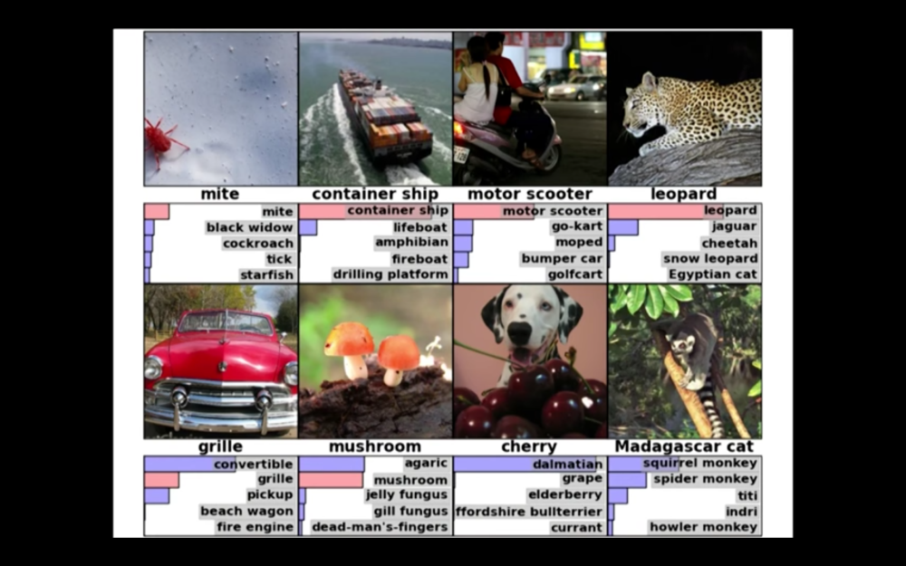
This was the first time in history that the neural net could actually do something.

Link to whole paper: Toronto ImageNet

HANDWRITING RECOGNITION:

Let us try to read this digit written by someone else:

2 ,seems easy right? Any literate person would look at this and immediately figure it out.

We carry in our heads a supercomputer, tuned by evolution over hundreds of millions of years, and superbly adapted to understand the visual world. Recognizing handwritten digits isn’t easy. Rather, we humans are stupendously, astoundingly good at making sense of what our eyes show us. But nearly all that work is done unconsciously.

But computers dont work that way, they have to go to through various data called as training examples inorder to make a decision when they encounter such handwritten digit again.

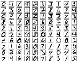
More the number of examples in training more would be the accuracy.

-Pratik Aher

NEXT UP: Working Module of neural network in python.